Note: The paragraph in the little dark color background represents small terms or concepts used in the main concept.

What is Naïve Bayes?

Naïve Bayes is a generative learning algorithm. It is a classification algorithm based on Bayes rule/theorem. The best area to use it is with discrete inputs such as text classification or categorical features. To understand Naïve Bayes, we first need to know Bayes rule/theorem and conditional probability.

Generative Learning Algorithms: Algorithms that try to learn p(y|x) directly (such as logistic regression), or algorithms that try to learn mappings directly from the space of inputs X to the labels {0, 1}, (such as the perceptron algorithm) are called discriminative learning algorithms. Here, we’ll talk about algorithms that instead try to model p(x|y) (and p(y)). These algorithms are called generative learning algorithms. For instance, if y indicates whether an example is a dog (0) or an elephant (1), then p(x|y = 0) models the distribution of dogs’ features, and p(x|y = 1) models the distribution of elephants’ features. - CS229 Lecture notes

The conditional probability of an event B is the probability that the event will occur given the knowledge that an event A has already occurred. This probability is written P(B|A), the notation for the probability of B given A. In the case where events A and B are independent (where event A does not affect the probability of event B), the conditional probability of event B given event A is simply the probability of event B, that is P(B). If events A and B are not independent, then the probability of the intersection of A and B (the probability that both events occur) is defined by P(A and B) = P(A) * P(B|A). - Yale

For example, in a positive and negative sentiment corpus, the probability of a positive sentence given that it has the word happy is:

Let’s continue with the above example to understand Bayes rule. Similar to the equation \(P(Positive | \text{"happy"}) = \frac{P(Positive \cap \text{"happy"})}{P(\text{"happy"})}\) in the above image, the probability of word happy given that the sentence is positive can be described as \(P(\text{"happy"} | Positive) = \frac{P(\text{"happy"} \cap Positive)}{P(Positive)}\).

Given both equations, we can now derive Bayes rule. Knowing that A∩B = B∩A, we can set both equations equals. After little calculation, we can rewrite it as

This is Bayes rule. Easy, right? In general, we write this equation as \(P(\text{X | Y}) = \frac{P(\text{Y | X}) P(X)}{P(Y)}\). Therefore, Bayes’ rule is based on the mathematical formulation of conditional probabilities. With Bayes’ rule, you can calculate the probability of X given Y if you already know the probability of Y given X and the ratio of the probabilities of X and Y.

Now, We know what Bayes’ theorem is. To model P(X|Y), we will, therefore, make a very strong assumption, which in reality is rarely the case. We will assume that the X_i’s are conditionally independent given Y. This assumption is called Naïve Bayes (NB) assumption, and the resulting algorithm is called Naive Bayes classifier.

In practice, P(X|Y) can be equal to zero in some cases, which causes problems in further calculations. To avoid P(X|Y) = 0, we use Laplacian smoothing. For example, in the sentiment text corpus example above, if our naive bayes model encounters any word that is not present in the corpus, then the model will output P(Positive | unknown) = 0 and P(Negative | unknown) = 0. The formula with example is given in the image below, where P(W_i | class) is probability of i^th word given the class. We add 1 to the numerator and add V to the denominator of naive bayes formula. The role of V here is to round the results such that total class probability sums up to 1.

In naive bayes inference, the ratios of the probability of positive words to the negative words is essential in naive bayes for binary classification. Using the sentiment example above, the blue box in below image represents the product of corresponding ratios of every word. If the result is > 1 then the sentence is positive, and if < 1, sentence sentiment is negative. This product of ratios, in the blue box, is called the likelihood. If we take the ratio between all positive and negative sentences, i.e. P(pos) / P(neg), it is known as the prior ratio, shown in the purple box in the image.

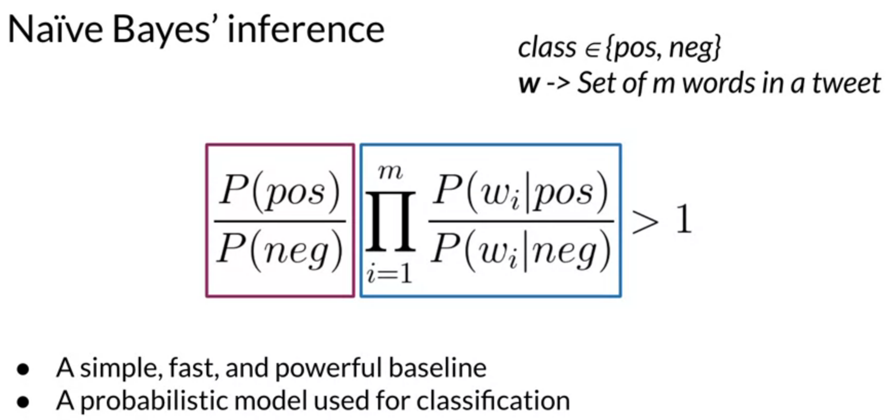
One more simplification is using log-likelihood instead of likelihood. The product of probabilities in likelihood can be close to zero if we take the product of many small probabilities. To overcome that, we use Log-likelihood to convert the product to sum. Below image shows the necessary details about the same.

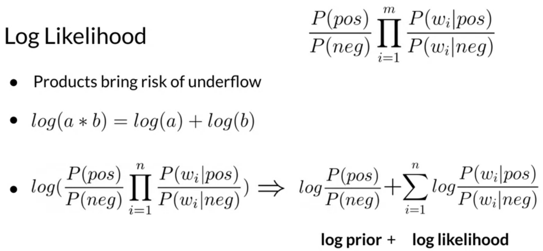
Likelihood and Log Likelihood: Watch 1, 2, 3, and 4 short videos for better understanding of likelihood.

Training Naïve Bayes

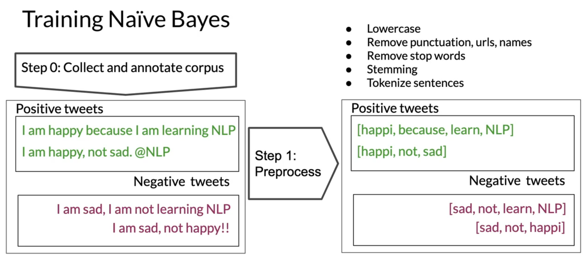
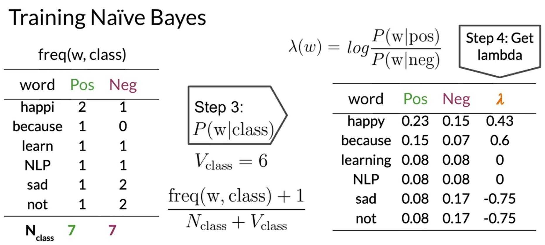
Now, let’s see how to train a Naïve Bayes model. Following are the steps to train a naïve bayes model:

1. Get or annotate a dataset with positive and negative tweets
2. Preprocess the tweets
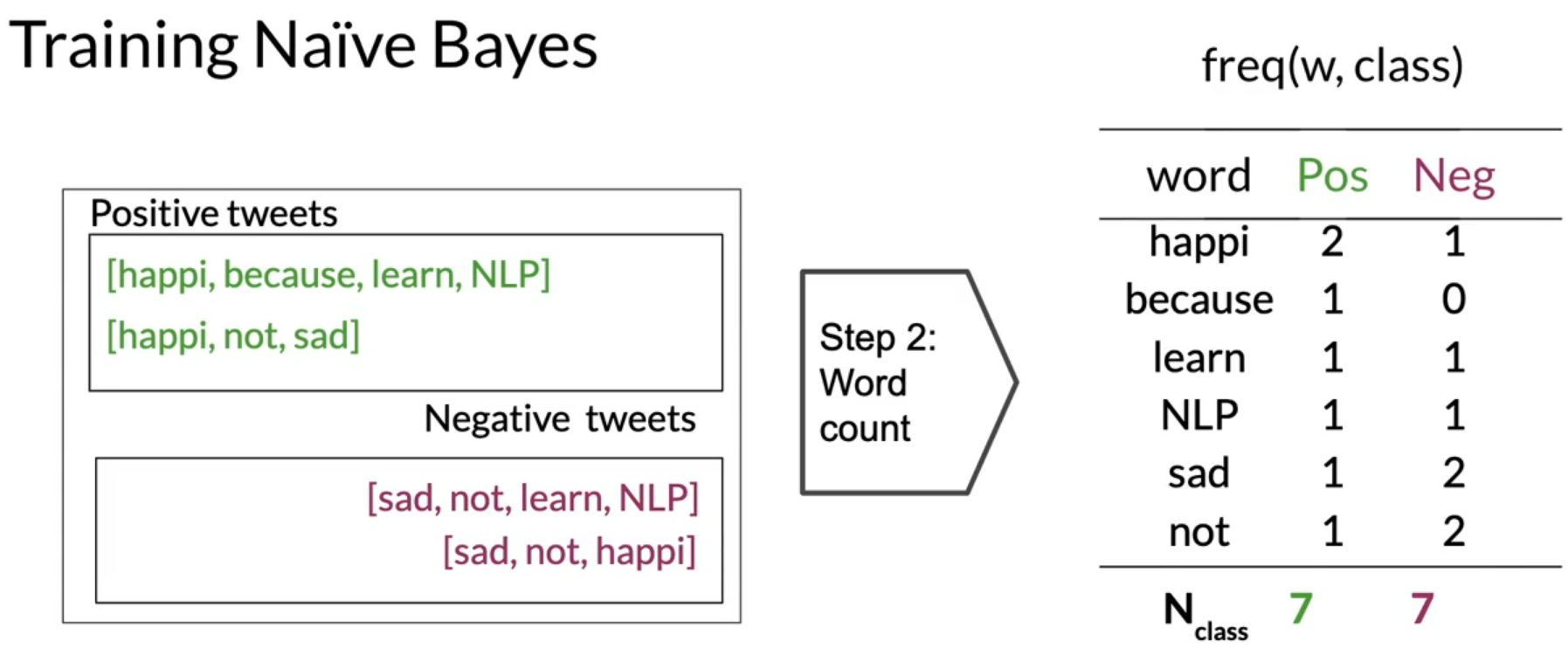
3. Compute freq of words with respect to class table, freq(w, class)
4. Get P(w | pos), P(w | neg)
5. Get log-likelihood dictionary \(\lambda (w) = log \frac{P(w \vert pos)}{P(w \vert neg}\)
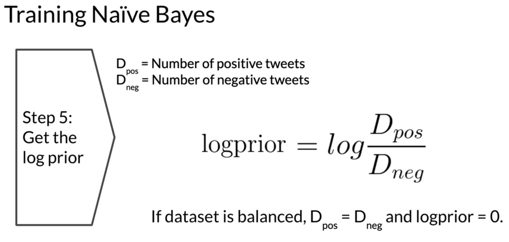
6. Compute \(logprior = log \frac{P(pos)}{P(neg)}\)

Let’s take an example of sentiment analysis to understand the above steps. Below images shows the steps-by-step process of training naive bayes for tweet sentiment analysis.

Testing Naïve Bayes

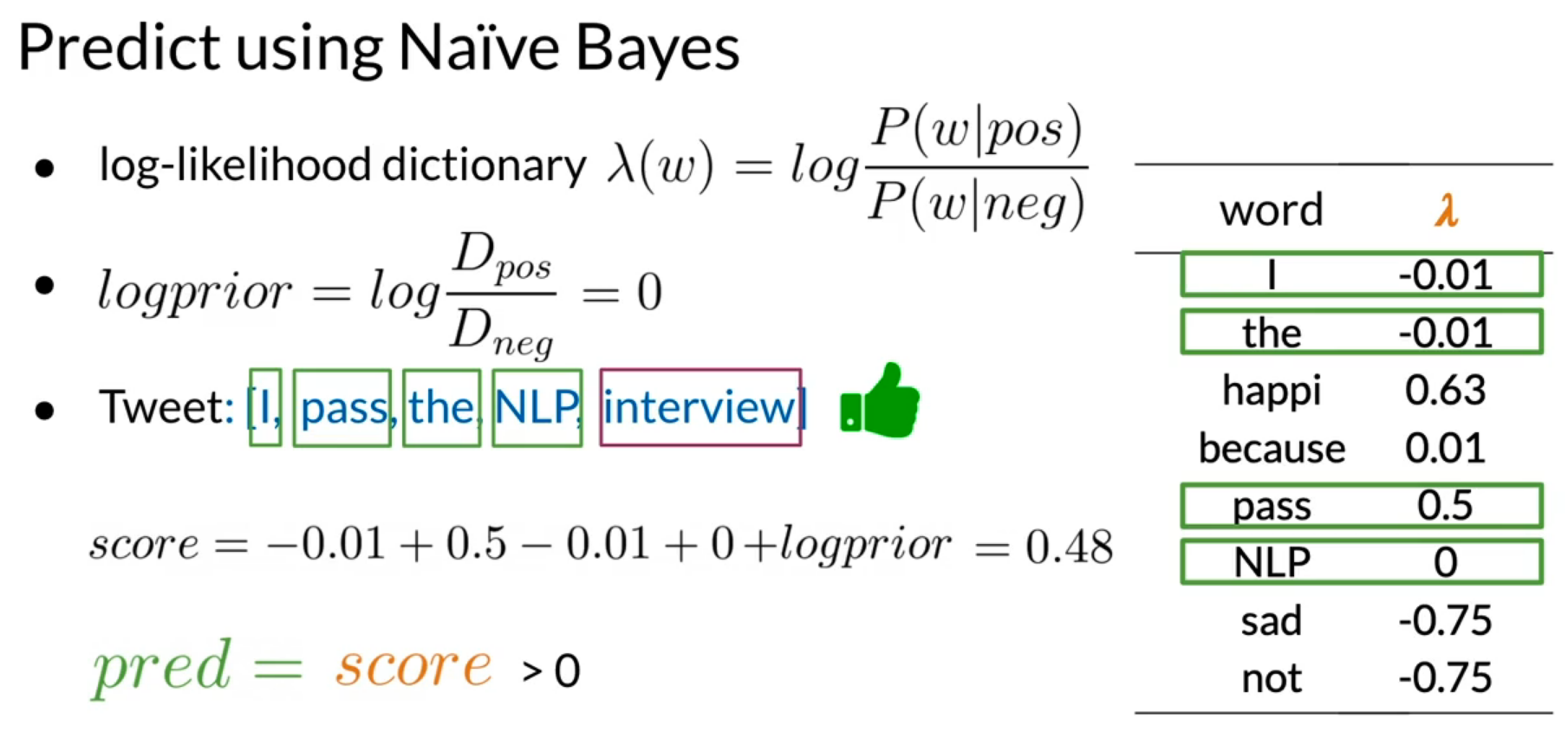
To test or predict new samples, we need learned \(\lambda (w)\) and \(logprior\). An example of tweet sentiment is shown in the image below. If the score is > 0 then tweet is positive. If score < 0 then tweet is negative. Note that, only words seen at training time will compute the score.

Where Naïve Bayes is useful?

Naïve Bayes performs better in:

• Sentiment analysis
• Author identification: Given a large corpus of different authors, naive bayes can distinguish them based on word frequencies.
• Spam filtering
• Information retrieval: finding out if a document is relevant or irrelevant to a given query. This can be achieved by computing the likelihood of each document.
• Word disambiguation: breaking down words for contextual clarity. Let’s say that you don’t know if the word Bank is referring to river or money. Now bank word can be used as bank of river or bank of money. To know the context of this particular word we can calculate \(\frac{P(river \vert text)}{P(money \vert text)}\). If the text refers to the river, then the score will be > 1. Similarly, if the text refers to the river, then the score will be < 1.

Where Naïve Bayes is NOT useful?

Naïve Bayes is not useful if the words are dependent in a sentence.

• One example of this problem is fill in the blanks. For example, It’s always cold and snowy in ____. And you have 4 options: spring, summer, fall, and winter. In this case, Naïve Bayes might assign equal probability to each word. Even though from the context you can see that the answer is winter. You might argue that, in the above section, we say that it is helpful in contextual clarity. Yes, but both are different cases. As said earlier, it might assign equal probabilities to each word. On the other hand, in word disambiguation, we have full text to compare.
• Another example is word order. Let’s take two sentences: I am happy because I did not go and I am not happy because I did go. Here the words are same and the model will assign same sentiment to both sentences.
• Removing words: If we remove the mutual/common words from sentence then the context might get confusing. For example, the sentence This is not good, because your attitude is not even close to being nice. after processing will return [good, attitude, close, nice] which indicates positive sentiment, whereas the actual sentence is negative.

References:

• Natural Language Processing with Classification and Vector Spaces Course - Coursera
• CS229 Lecture notes
• Yale